HKUST CSIT5401 Recognition System lecture notes 2. 识别系统复习笔记。
Introduction
Face recognition and iris recognition are non-invasive method for verification and identification of people. In particular, the spatial patterns that are apparent in the human iris are highly distinctive to an individual.
Schematic diagram of iris recognition
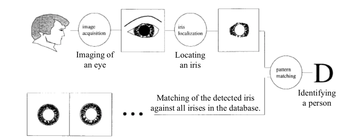
Image Acquisition Systems
One of the major challenges of automated iris recognition is to capture a high-quality image of the iris while remaining non-invasive to the human operator.
There are three concerns while acquiring iris images:
- To support recognition, it is desirable to acquire images of the iris with sufficient resolution and sharpness.
- It is important to have good contrast in the interior iris pattern without resorting to a level of illumination that annoys the operator, i.e., adequate intensity of source constrained by operator comfort with brightness.
- These images must be well framed (i.e., centered) without unduly constraining the operator.
The Daugman system
The Daugman system captures images with the iris diameter typically between 100 and 200 pixels from a distance of 15-46cm.
The system makes use of an LED-based point light source in conjunction with a standard video. By carefully positioning of the point source below the operator, reflections of the light source off eyeglasses can be avoided in the imaged iris.
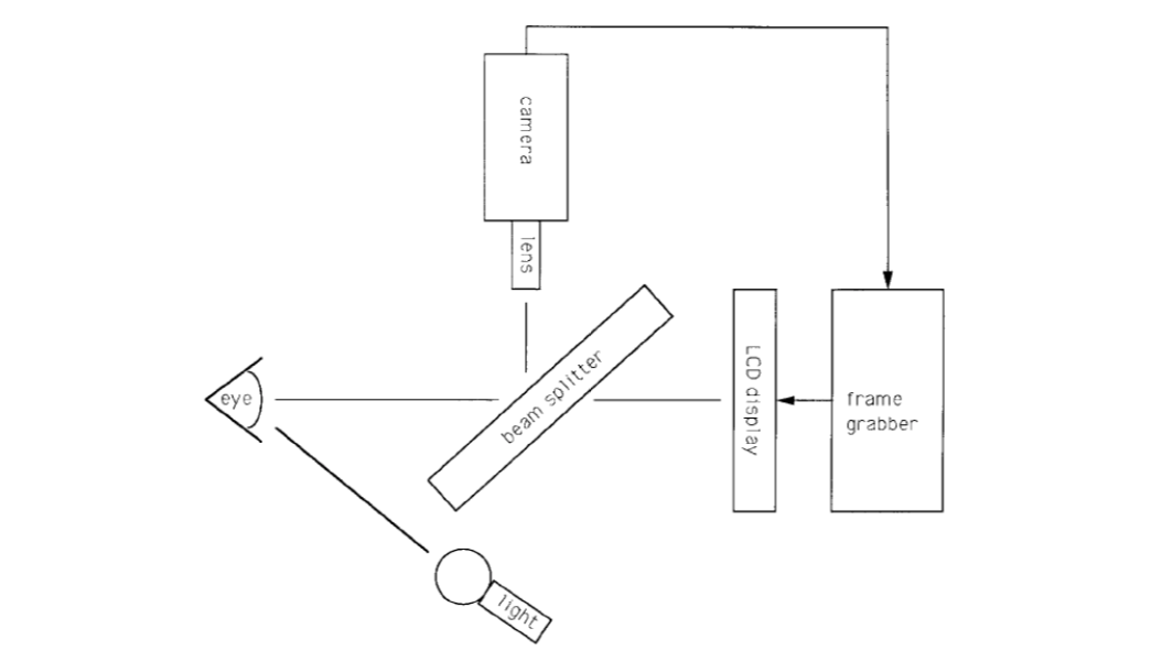
The Daugman system provides the operator with live video feedback via a tiny liquidcrystal display placed in line with the camera's optics via a beam splitter. This allows the operator to see what the camera is capturing and to adjust his position accordingly.
The Wildes system
The Wildes system images the iris with approximately 256 pixels across the diameter from 20cm. The system makes use of a diffused source and polarization in conjunction with a low-light level camera.
The use of matched circular polarizer at the light source and camera essentially eliminates the specular reflection of the light source.
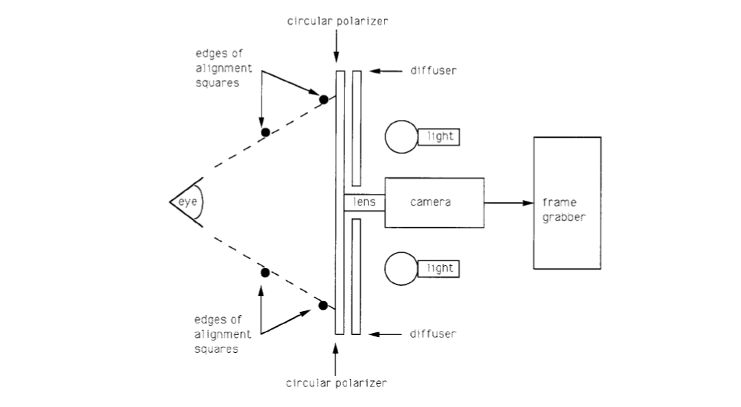
The coupling of a low light level camera with a diffused illumination allows for a level of illumination that is entirely unobjectionable to human operators.
The relative sizes and positions of the square contours are chosen so that when the eye is in an appropriate position, the squares overlap and appear as one to the operator.
Iris localization
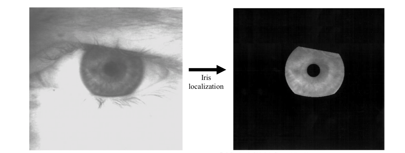
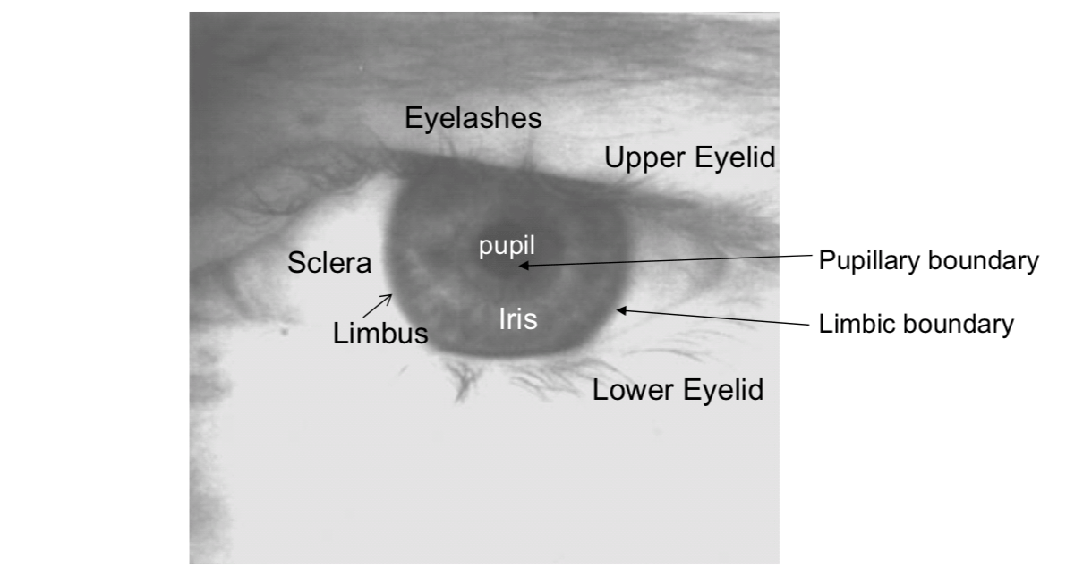
Image acquisition will capture the iris as part of a larger image that also contains data derived from the immediately surrounding eye region. For example, eyelashes, upper eyelid, lower eyelid and sclera. Therefore, prior to performing iris pattern matching, it is important to localize that portion of the acquired image that corresponds to an iris.
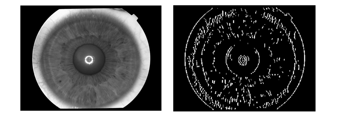
The Wildes system makes use of the first derivatives of image intensity to signal the location of edges that correspond to the borders of the iris.
- Step 1: The image intensity information is converted into binary edge-map.
- Step 2: The edge points vote to particular contour parameter values.
Step 1
The edge map is recovered via gradient-based edge detection. This operation consists of thresholding the magnitude of the image intensity gradient magnitude. \(I\) is the intensity and (x, y) are the image coordinates. \[
\text{Gradient magnitude }|\triangledown G(x, y)\ast I(x, y)|\\
\text{2D Gaussian function } G(x, y)=\frac{1}{2\pi\sigma^2}\exp(\frac{(x-x_0)^2+(y-y_0)^2}{2\sigma^2})
\] 
Step 2
The voting procedure is realized via the Hough transform. For circular limbic or pupillary boundaries and a set of recovered edge points, a Hough transform is defined as follows.
Edge points \((x_j, y_j)\) for \(j = 1, ..., n\): \[
H(x_c, y_c, r)=\sum_{j=1}^nh(x_j,y_j,x_c,y_c,r)
\] where \[
h(x_j, y_j, x_c, y_c, r)=\begin{cases}
1, \text{ if }\ g(x_j, y_j, x_c, y_c, r)=0\\
0, \text{ otherwise}
\end{cases}\\
g(x_j, y_j, x_c, y_c, r)=(x_j-x_c)^2+(y_j-y_c)^2-r^2
\] For every parameter triple \((x_c, y_c, r)\) that represents a circle through the edge point \((x_j, y_j)\), \[
g(x_j, y_j, x_c, y_c, r)=0
\] 
The parameter triple that maximizes the Hough space \(H\) is common to the largest number of edge points and is a reasonable choice to represent the contour of interest.
The limbus and pupil are modeled with circular contour models.
The Daugman system fits the circular contours via gradient ascent on the parameters so as to maximize \[ \left|\frac{\partial}{\partial r}G(r)\ast\oint_{x_c,y_c,r}\frac{I(x,y)}{2\pi r}ds\right| \] where \(G(r)=\frac{1}{\sqrt{2\pi}\sigma}\exp(-\frac{(r-r_0)^2}{2\sigma^2})\); \(r_0\) is the center.
The first part of the equation is to perform Gaussian smoothing; while the second part is computing the average intensity along the circle.
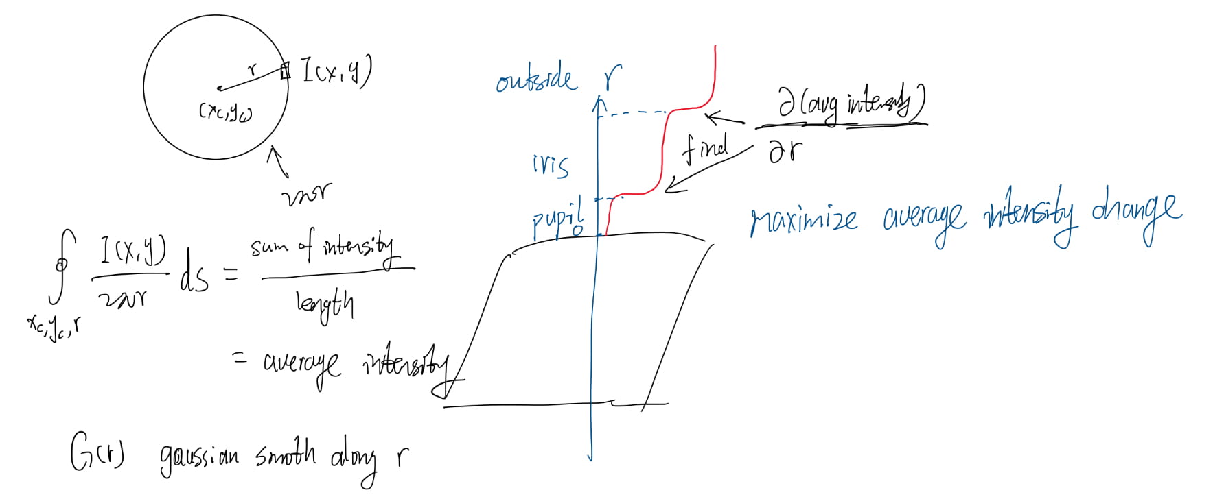
In order to incorporate directional tuning of the image derivative, the arc of integration \(ds\) is restricted to the left and right quadrants (i.e., near vertical edges) when fitting the limbic boundary.
This arc is considered over a fuller range when fitting the pupillary boundary.
Pattern Matching
Having localized the region of an acquired image that corresponds to the iris, the final task is to decide if this pattern matches a previously stored iris pattern.
There are four steps:
- Alignment: bringing the newly acquired iris pattern into spatial alignment with a candidate data base entry.
- Representation: choosing a representation of the aligned iris patterns that makes their distinctive patterns apparent.
- Goodness of Match: evaluating the goodness of match between the newly acquired and data base representations.
- Decision: deciding if the newly acquired data and the data base entry were derived from the same iris based on the goodness of match.
Alignment (Registration)
To make a detailed comparison between two images, it is advantageous to establish a precise correspondence (or matching) between characteristic structures across the pair.
Both systems (Daugman and Wildes systems) compensate for image shift, scaling and rotation.
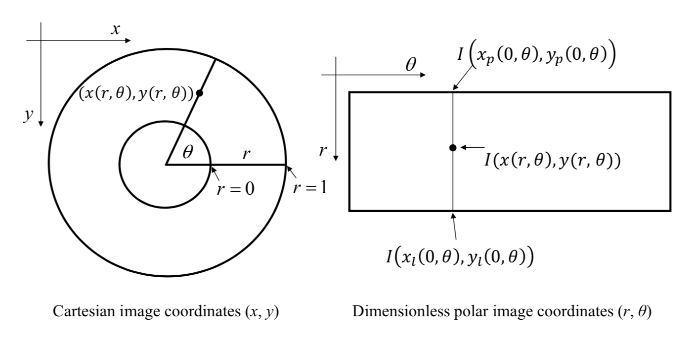
The Daugman system for alignment
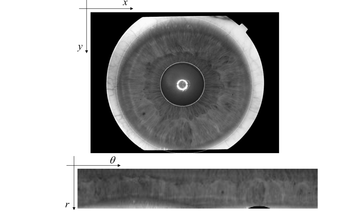
The Daugman system uses radial scaling to compensate for overall size as well as a simple model pupil variation based on linear stretching.
The system maps the Cartesian image coordinates \((x, y)\) to dimensionless polar image coordinates \((r, θ)\) according to \[
x(r,\theta)=(1-r)x_p(0,\theta)+rx_l(1,\theta)\\
y(r,\theta)=(1-r)y_p(0,\theta)+ry_l(1,\theta)
\] 
The Wildes system for alignment
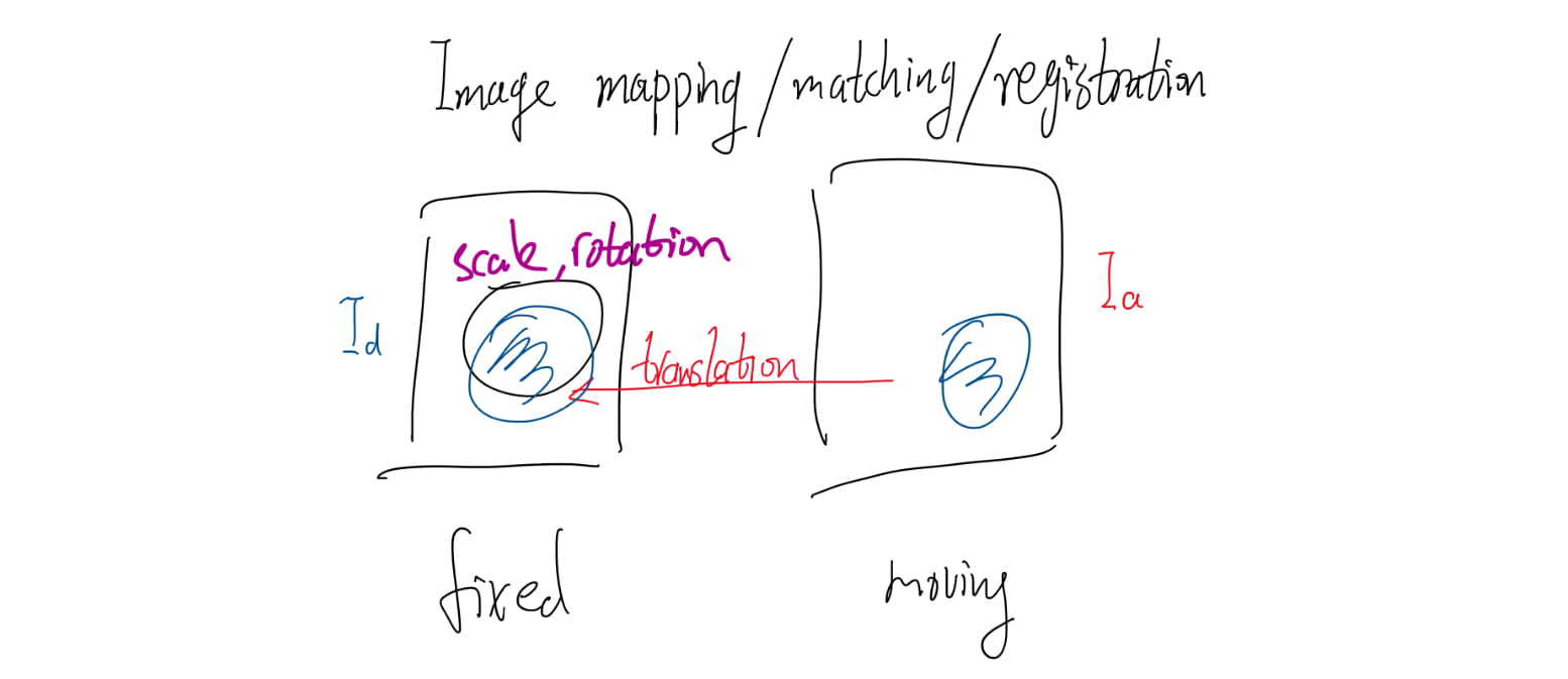
The Wildes system uses an image-registration technique to compensate for both scaling and rotation.
This approach geometrically warps a newly acquired image \(I_a (x, y)\) into alignment with a selected data base image \(I_d (x, y)\) according to a mapping function \((u(x, y), v(x, y))\) such that for all \((x, y)\), the image intensity value at \((x, y) – (u(x, y), v(x, y))\) is close to that at \((x, y)\) at \(I_d\).
The mapping function is taken to minimize \[ \int_x\int_y\left(I_d(x,y)-I_a(x-u, y-v)\right)^2dxdy \] under the constrains to capture similarity transformation of image coordinates \((x,y)\) to \((x'=x-u, y'=y-v)\).
Translation \[
\vec{x}'=\vec{x}+\vec{d}
\] ![]()
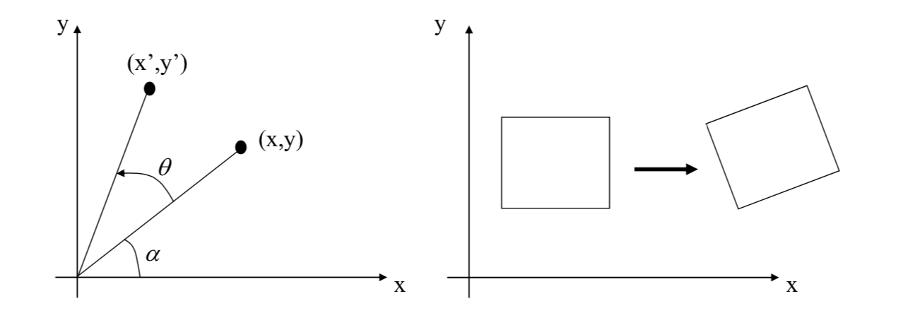
Rotation \[
\vec{x}'=R_\theta\vec{x}\\
R_\theta=\begin{pmatrix}
\cos\theta & -\sin\theta \\
\sin\theta & \cos\theta
\end{pmatrix}
\] 
Rotation + Translation \[
\vec{x}'=R\vec{x}+\vec{d}
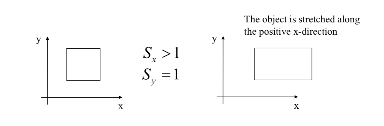
\] Scaling + Translation \[
\vec{x}'=S\vec{x}+\vec{d}
\] 
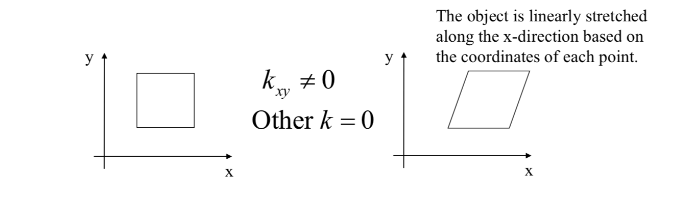
Shearing \[
\vec{x}'=K\vec{x}\\
K=\begin{bmatrix}
1 & k_{xy} \\
k_{yx} & 1
\end{bmatrix}
\] 
Affine: translation + rotation + scaling + shearing \[ \vec{x}'=R_\theta S K\vec{x}+\vec{d} \] Example: \[ \begin{bmatrix} x' \\ y' \end{bmatrix}=\begin{bmatrix} \cos\theta & -\sin\theta \\ \sin\theta & \cos\theta \end{bmatrix}\begin{bmatrix} s_x & 0 \\ 0 & s_y \end{bmatrix}\begin{bmatrix} 1 & k_{xy} \\ k_{yx} & 1 \end{bmatrix}\begin{bmatrix} x \\ y \end{bmatrix}+\begin{bmatrix} d_x \\ d_y \end{bmatrix} \]
Representation
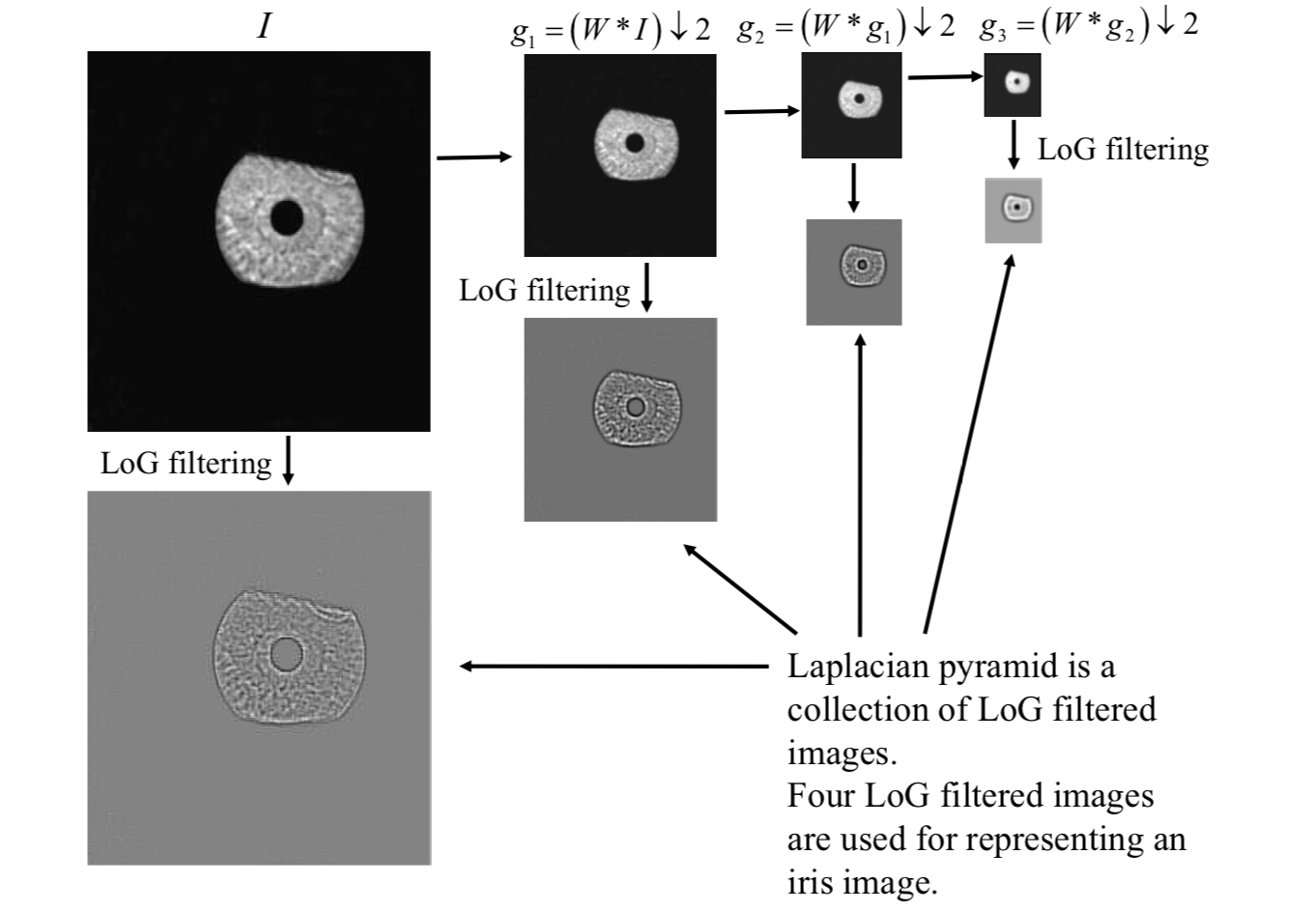
To represent the iris image for matching, both the Daugman and Wildes systems capture the multiscale information extracted from the image.
The Wildes system makes use of the Laplacian of Gaussian filters to construct a Laplacian pyramid.
The Laplacian of Gaussian (LoG) filter is given by \[ -\frac{1}{\pi\sigma^4}\left(1-\frac{\rho^2}{2\sigma^2}\right)\exp(-\frac{\rho^2}{2\sigma^2}) \] where \(\rho\) is radial distance of a point from the filter's center; \(\sigma\) is standard deviation.
A Laplacian pyramid is formed by collecting the LoG filtered images.
Goodness of Match
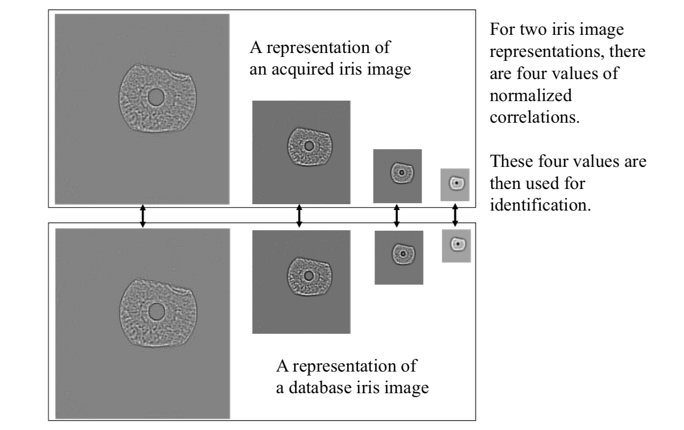
The Wildes system uses the normalized correlation between the acquired representation and data base representation. In discrete form, the normalized correlation can be defined as follows.
Let \(p_1[i, j]\) and \(p_2[i, j]\) be two image arrays of size \(n \times m\).
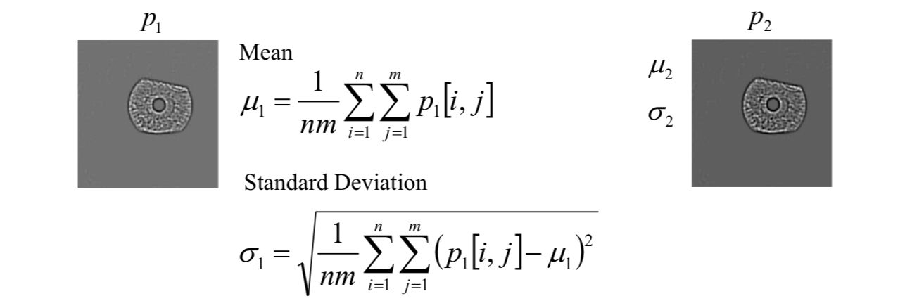
The normal correlation is \[
NC=\frac{\sum_{i=1}^n\sum_{j=1}^m(p_1[i,j]-\mu_1)(p_2[i,j]-\mu_2)}{nm\sigma_1\sigma_2}
\] 
Decision (FLD)
The Wildes system combines four estimated normalized correlation values into a single accept/reject judgment.
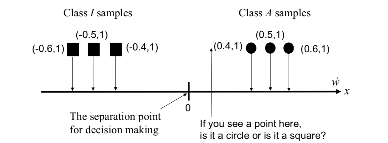
In this application, the concept of Fisher's linear discriminant is used for making binary decision. A weight vector is found such that the variance within a class of iris data is minimized while the variance between different classes of iris data is maximized for the transformed samples.
In iris recognition application, usually there are two classes: Authentic class (A) and Imposter class (I).
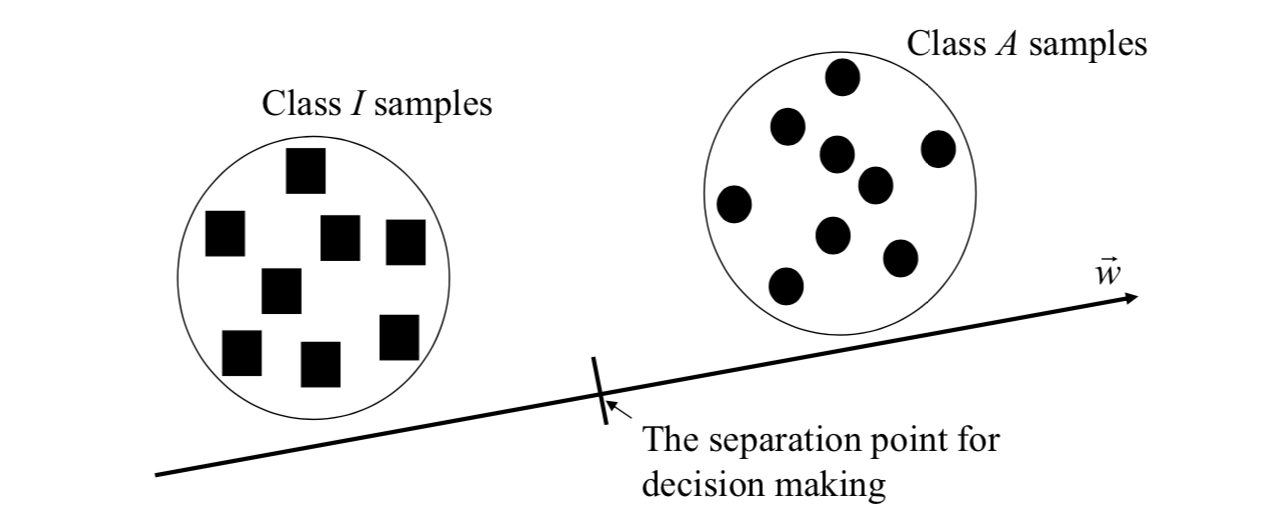
To make a binary decision on a line, all points are projected onto the weight vector (or samples are transformed by using the weight vector).
In iris recognition using the Wildes system, all samples are 4-dimensional vectors. Let there be n 4-dimensional samples.
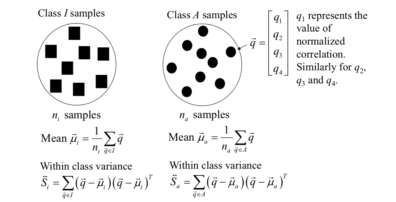
The total within class variance is \[ \vec{S}_w=\vec{S}_i+\vec{S}_a \] Between class variance is \[ \vec{S}_b=(\vec{\mu}_a-\vec{\mu}_i)(\vec{\mu}_a-\vec{\mu}_i)^T \] If all samples are transformed, the ratio of between class variance to total within class variance is \[ \frac{\vec{w}^T\vec{S}_b\vec{w}}{\vec{w}^T\vec{S}_w\vec{w}} \] The ratio is maximized when \[ \vec{w}=\vec{S}_w^{-1}(\vec{\mu}_a-\vec{\mu}_i) \] And the separation point for decision making is \[ \frac{1}{2}\vec{w}^T(\vec{\mu}_a+\vec{\mu}_i) \] Therefore, values above this point will be taken as derived from class \(A\); values below this point will be taken as derived from class \(I\).
Hough Transform
Detecting Lines
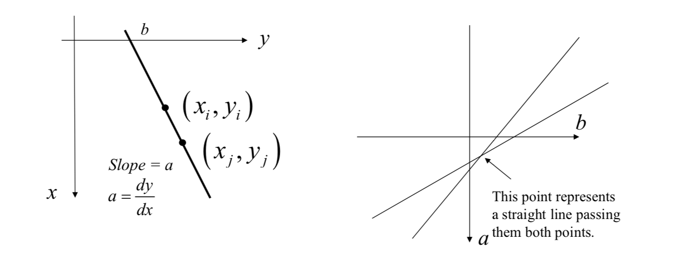
Idea: if two edge points \((x_i, y_i)\) and \((x_j, y_j)\) lie on the same straight line, then they should have the same values of slope and y-intercepts on the xy-plane.
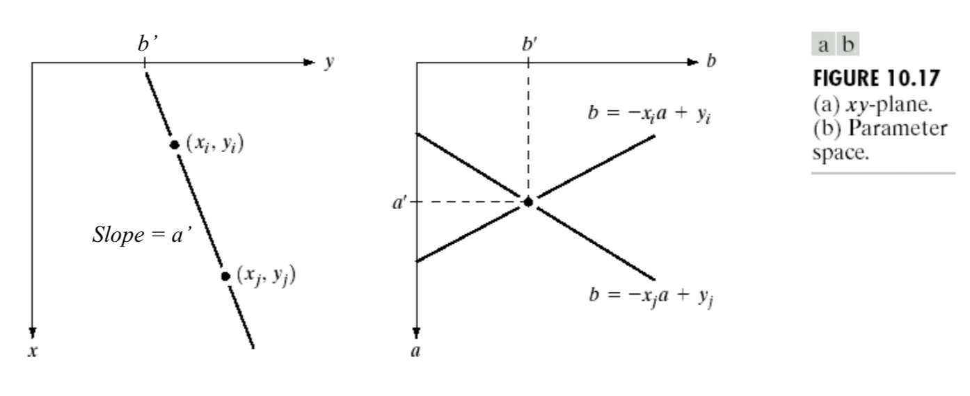
[1] For a point \((x_i,y_i)\), we set up a straight line equation: \[ y_i=ax_i+b\Leftrightarrow b=(-x_i)a+y_i \] where \(a\) = slope, \(b\) = y-intercept, \(x_i\) and \(y_i\) are known and fixed.
[2] We subdivide the a axis into \(K\) increments between \([a_\min,a_\max]\). For each increment of \(a\), we evaluate the value of \(b\).
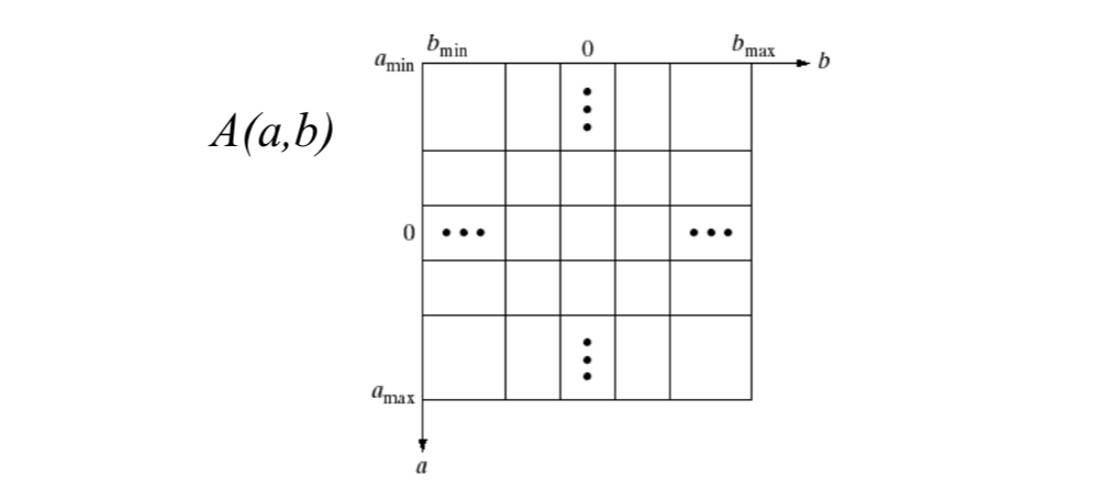
[3] A relationship between \(a\) and \(b\) can be plotted in a parameter space, i.e., ab-plane.
[4] We partition the parameter space into a number of bins (accumulator cells), and increment the corresponding bin \(A(a,b)\) by 1 (\(b\) is rounded into the nearest integer).
[5] For another point \((x_j,y_j)\), we set up another straight line equation: \[ y_j=ax_j+b\Leftrightarrow b=(-x_j)a+y_j \] [6] Similarly, we subdivide the a axis into K increments between \([a_\min,a_\max]\). For each increment of \(a\), we evaluate the value of \(b\). We plot the relationship between \(a\) and \(b\) in the same parameter space, and update bin values in the discrete parameter space.
[7] The bin \(A(a,b)\) having the highest count corresponds to the straight line passing through the points \((x_i,y_i)\) and \((x_j,y_j)\).
[8] The same procedure can be applied to all points. The bin \(A(a,b)\) having the highest count corresponds to the straight line passing through (or passing near) the largest number of points.
Problem: Values of \(a\) and \(b\) run from negative infinity to positive infinity. We need infinite number of bins!
Solution: use normal representation of a line: \[
x\cos(\theta)+y\sin(\theta)=\rho
\] 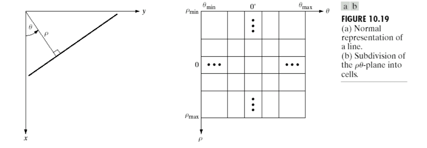
\(\theta\) runs from \(–90^o\) to \(90^o\). \(\rho\) runs from \(-\sqrt{2}D\) to \(\sqrt{2}D\), where \(D\) is the distance between corners in the image (length and width).
Circle Hough Transform (CHT)
The Hough transform can be used to determine the parameters of a circle when a number of points that fall on the perimeter are known. A circle with radius \(R\) and center \((a, b)\) can be described with the parametric equations: \[ x=a+R\cos(\theta)\\ y=b+R\sin(\theta) \] When the angle \(θ\) sweeps through the full 360 degree range the points \((x, y)\) trace the perimeter of a circle.
If the circles in an image are of known radius \(R\), then the search can be reduced to 2D. The objective is to find the \((a, b)\) coordinates of the centers.
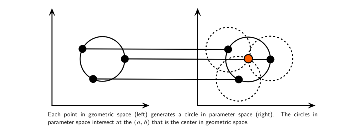
If the radius is not known, then the locus of points in parameter space will fall on the surface of a cone. Each point \((x, y)\) on the perimeter of a circle will produce a cone surface in parameter space. The triplet \((a, b, R)\) will correspond to the accumulation cell where the largest number of cone surfaces intersect.
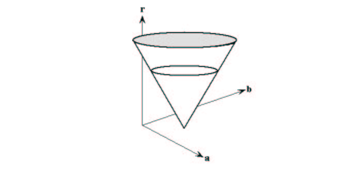 The drawing above illustrates the generation of a conical surface in parameter space for one \((x, y)\) point. A circle with a different radius will be constructed at each level, \(r\).
The search for circles with unknown radius can be conducted by using a three dimensional accumulation matrix.